Faster simulation of self-avoiding walks promises to untangle knotty problems in polymer science
by Jason Whyte (April, 2016).
This feature article describing my research into fast simulations of self-avoiding walks can also be read as a pdf file. (The formatting in the pdf file is much better; the html displayed here is a shoddy conversion which will be tidied up sometime in the future.)
Jason is currently (as of November 2016) completing a PhD in mathematics at the University of Melbourne. You can find scientific articles he has authored at his Google Scholar page.
Summary
First proposed by Orr in 1947, the mathematical notion of a `self-avoiding walk' (SAW) is simple to define, yet incredibly useful to the understanding of particular types of physical phenomena. For example, under certain conditions, SAWs can exactly model some properties of polymers — long chains of fundamental units (monomers) held together by chemical bonds. SAWs are not only a useful modelling tool; over decades their study has stimulated theoretical developments in areas including mathematics, physics and computer science.
The challenging problems posed by SAWs have drawn the interest of winners of the Fields medal, an award considered the equivalent of a Nobel Prize in the discipline of mathematics. Researchers from The School of Mathematics and Statistics at The University of Melbourne have a history of making contributions to the study of SAWs. In continuing this record, Dr Nathan Clisby was awarded a prestigious Future Fellowship by the Australian Research Council to foster his research into the efficient simulation of SAWs. These awards enable outstanding mid-career researchers to continue their research in Australia. Nathan's work underpins advances in certain branches of mathematics and physics. It also promises insight into long-unexplained phenomena, such as knotting in polymers.
Self-avoiding walks, polymers and stubborn mathematical problems
We begin our overview of the contributions made by Nathan’s research to the study of self-avoiding walks (SAWs) with a summary of their properties.
An introduction to SAWs
A SAW occurs on a ‘regular lattice’ of some fixed dimension d in which points are spaced evenly according to some rule. Figure 1 shows one regular lattice in each of two dimensions (d = 2) and three dimensions (d = 3). Other regular lattices for d = 2 are comprised of repeating shapes such as triangles or hexagons, and extensions exist for higher dimensions.
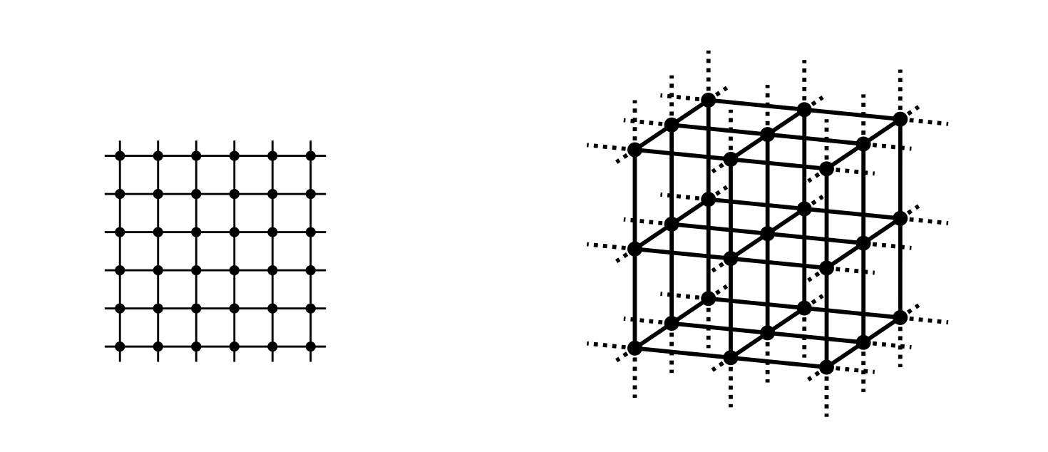
Figure 1: A square lattice (d=2, left) and a simple cubic lattice (d=3, right).
An n-step SAW (where n will always represent a positive integer) is a sequence of n + 1 distinct lattice points ω0, ω1, …, ωn, each a nearest neighbour of its predecessor. We can think of these points as defining a path (or conformation) traced out on a regular lattice by a pipe cleaner that is subject to constraints. One end — representing the ‘zeroth’ monomer — is placed at the lattice’s origin (this defines ω0). The pipe cleaner is bent some integer number of times (between 0 and n inclusive) to make a path through n lattice points that are nearest neighbours. Vitally, the pipe cleaner cannot intersect itself. The position of the end furthest from the origin (ωn) gives the location of the n-th monomer. Figure 2a shows an example of a SAW on a square lattice.
If the n + 1 lattice points ω0, ω1, …, ωn are not required to be distinct, the sequence defines an ‘n-step random walk’ . From a starting point ω0, the walk takes its first step to ω1, a lattice point that is a nearest neighbour. It continues stepping in this manner for a total of n steps and may visit a point one or more times. A random walk has the ‘Markovian’ property, which allows its simulation in a stepwise manner. That is, the only information we need to simulate the next step of the walk is its current location. Figure 2b shows an example of a simple random walk. SAWs do not have the Markovian property, which makes their simulation more complicated than that of random walks.
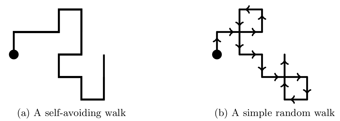
Figure 2: The figures use a square lattice to show an example of each of (a) a self-avoiding walk and (b) a simple random walk. In each case the filled circle shows $\omega_0= (0,0)$, the lattice's origin. While arrows are useful for showing the progress of a random walk from the origin, they are inappropriate for a SAW.
The number of distinct n-step SAWs conformations on some regular
lattice is represented by cn. For n tending towards infinity, it
is widely believed that cn follows the
(asymptotic) relation1
$$\begin{aligned}
c_n \sim A \mu^n n^{\gamma -1},
\label{eq:c_n}\end{aligned}$$
where constant A and ‘growth constant’ μ depend on the type of lattice. The
‘critical exponent’ γ depends
only on d. For example, it is
expected that for large n the
expressions for cn on a square lattice
and a hexagonal lattice have the same μ value as for both d = 2. While the dependency of cn on μn is
established, the existence of γ has not yet been proven for 2 ≤ d ≤ 4.
By knowing each of the cn conformations of n-step SAWs, we can calculate some property (‘observable’) of this set. One example is the ‘mean square size’ of SAWs (average square end-to-end distance) represented by $\langle {\rm R^{2}_{e}} \rangle_n$. This is obtained by determining the distance of the n-th monomer from the origin for each conformation, squaring this value, and averaging the set of values. It is believed that as n tends to infinity we have the asymptotic relationship
$$\begin{aligned}
\langle {\rm R^{2}_{e}} \rangle_n \sim D n^{2\nu},
\label{eq:mean_length}\end{aligned}$$
where ν is a universal constant for a
given d and is regarded as
another critical exponent. The constant D depends on the lattice type. The strong
conviction that the above asymptotic relationships are correct has led to much research
aimed at determining the critical exponents γ and ν. This requires values (or at least good
estimates) of cn and $\langle {\rm
R^{2}_{e}} \rangle_n $ for large n as inputs to the estimation process. We must
overcome some very difficult problems in order to obtain this
information.
To gain some appreciation for such problems and the means of addressing them, we give an overview of polymers, an early application of SAWs proposed by Flory in 1949.
An introduction to features of polymers
Polymers feature in many industries and products. Two examples are polyethylene used in garden chairs, and paint used to protect steel from rust. Biological polymers include DNA, the store of genetic information required for an organism’s reproduction. Two simplified polymer structures are shown in Figure 3.
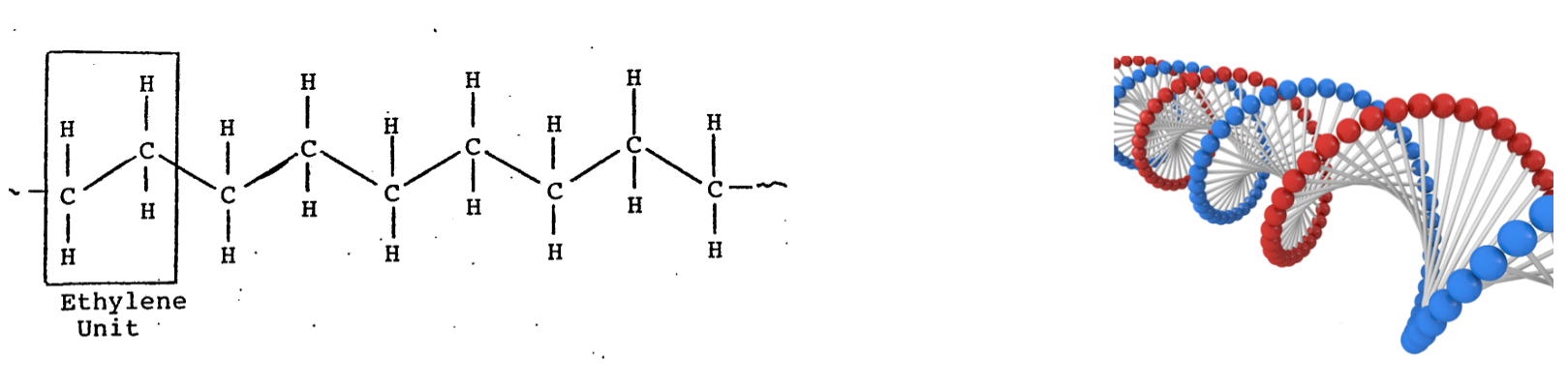
Figure 3: The chemical structure of polyethylene, highlighting its repeating unit (left) and a simplified structure of double-stranded DNA (right, blue and red spheres represent monomers). (DNA image from [1])
A polymer may have millions or even billions of monomers. Forces due to these influence a polymer’s shape (generally ‘conformation’). Their effect is subject to the polymer’s environment; this may be an industrial solvent or the cytoplasm of a cell. Conformation influences a polymer’s properties. For example, compared to an enzyme’s ideal conformation, a mis-folded version may have a decreased ability to catalyse a chemical reaction. Varied consequences in humans include Alzheimer’s disease ([2]).
The surprisingly profitable connection between polymers and SAWs
SAWs exactly model certain features of ‘isolated polymers’. These are polymers in dilute solution in a ‘good solvent’, one that negates the attractive forces between non-adjacent monomers. As a result, multiple monomers do not occupy the same region of space. This creates an ‘excluded volume effect’, causing the polymers to spread out in the solvent volume much more than they would otherwise. This characteristic gives some intuitive motivation for the modelling of a polymer conformation with a SAW.
The study of isolated polymers in solution has provided experimental justification for modelling their properties with SAWs. For example, light scattering experiments have estimated the mean size of polymers (average end-to-end distance) of a known number of monomers n. These experiments were performed for multiple n. Results obtained gave an empirical relationship for how mean square polymer size grows with n. For large n, mean square size grows with a factor of n2ν, as was proposed for mean square size of n-step SAWs. The experimentally-derived estimate of ν is limited to two decimal place accuracy. However, it is in agreement with the estimate of ν to five decimal places calculated using Nathan’s methods applied to n-step SAWs with appropriate n values. This agreement between experimental and computationally-derived values holds regardless of the type of lattice used as long it is in three dimensions, and regardless of the isolated polymer’s composition.
The ability of SAWs — a simple model that does not attempt to model physical features in detail — to exactly capture properties of isolated polymers exemplifies a useful property. That is, certain systems exhibit properties that change with n (say, number of steps or monomers) according to the same critical exponent. These systems are said to belong to the same ‘universality class’. The ability of mathematical systems to provide insights into properties of real systems from the same universality class is a powerful technique in research into ‘critical phenomena’.
Practicalities of the use of SAWs in estimating the properties of physical systems
Determining cn for SAWs on a one-dimensional (d = 1) regular lattice (points on a straight line) is trivial. An n-step SAW with one end at the origin can only have the other end either n lattice points to the left or right. Hence, cn = 2 for any n. However, the problem of calculating cn for large n — or even obtaining a good estimate for it — for lattices of interest to physical applications is much more complex.
For lattices with d = 2 or d = 3 (recall the examples shown in Figure 1), for small values of n we can count the n-step SAWs directly to determine cn. However, counting becomes impractical for relatively small n. Hence, it is necessary to simulate SAWs with the aim of obtaining a good approximation to cn. The nature of SAWs poses certain difficulties for such simulations. Unlike a random walk, it is difficult to simulate a SAW in a stepwise manner. One difficulty is that of ‘trapping’; after k < n steps we may arrive at a conformation for which no further step is possible. This possibility makes stepwise simulation of n-step SAWs inefficient as computational effort is spent without obtaining a valid conformation. As a result, much research has gone into simulation methods more likely to produce SAWs for large n.
Challenges and opportunities in the study of SAWs
The ‘hard counting problem’ of exactly determining cn for general n and fixed d and lattice type has been studied for more than 60 years. The problem may be ‘unsolvable’ in the sense that there may not exist a ‘nice’ expression for cn.2 Whether the problem is unsolvable or not is an open question. This makes the problem of continuing interest to communities of mathematicians and physicists. To them it is an intrinsically interesting and rich problem quite apart from any physical applications.
The problem of obtaining cn has stimulated research in various areas. Efforts in the field of combinatorics are aimed at improving approximations to cn. This in turn has prompted the development of enumeration algorithms in computer science. Probability theory has incorporated ideas from SAWs in the development of the concepts of ‘lace expansion’ and ‘Stochastic Löwner Evolution’. SAWs are also a limiting case of the ‘n-vector models’ proposed to explain aspects of the behaviour of materials. For n = 1 this model class yields the famous Ising model of ferromagnetism which is central to the theory of critical phenomena.
In terms of applications, the study of SAWs has impacted various areas, including polymer physics, chemistry, and materials science. These disciplines have considered polymer systems, including branched and ring polymers, to investigate properties such as the distribution of polymer sizes. SAWs do not attempt to model the chemistry that influences the conformations of non-isolated polymers. However, this effect is included in more sophisticated models that build on the framework provided by SAWs, such as the HP (hydrophobic) model.
In biology, models related to SAWs are suitable for studying or representing processes such as protein folding3 and the folding of RNA enclosed by a viral capsid. Another application, understanding the knotting of DNA, is a particular challenge for methods of simulating SAWs. Polymer knotting only becomes common when the number of constituent monomers is of the order of millions. Until relatively recently, algorithms for simulation of SAWs with correspondingly large n were impractical. This was due to algorithms requiring prohibitively long run times to produce results sufficiently accurate to be useful. Nathan’s work has overcome this difficulty by reformulating the problem.
The next section considers the problem of simulating SAW conformations in detail. We will subsequently outline the development of some techniques used for this purpose. Finally, we will take an overview of Nathan’s innovative refinements which make great strides in the simulation of self-avoiding walks.
Algorithms for SAW simulation and the need for speed
An important feature of any algorithm is the number of computer operations it takes to complete a task. This number is directly related to the algorithm’s run time. If one algorithm uses fewer operations than another to achieve a comparable result, it is considered more efficient.
There are a variety of algorithms for the computer simulation of SAW conformations. We will describe a type that features prominently in Nathan’s research, and progress with making these more efficient.
Markov Chain Monte Carlo methods for simulation of SAWs
Suppose that each n-step SAW configuration on some regular lattice is called a ‘state’ and the entire collection of these is a ‘state space’. This formulation allows us to consider algorithms that produce SAW conformations by using Markov Chain Monte Carlo (MCMC) simulation.4 They provide a means of drawing a number of states from the state space. This is termed ‘sampling from the state space’. We will give a general description of such algorithms applied to our context.
A MCMC-type algorithm begins with an initial n-step SAW conformation. This, and any subsequent conformation, is stored in computer memory through a particular value of a ‘data structure’. Typically this is a table which encodes the position on the lattice occupied by each of the n + 1 monomers. The first step of the algorithm is to deform the initial configuration via a ‘move’ chosen at random. Any move has two possible results. If the result is a SAW it is ‘accepted’ and becomes the updated conformation. The data structure is modified to record this new conformation. Otherwise, the result is ‘rejected’ and the initial conformation becomes the updated conformation, requiring no change to the data structure. Regardless of whether the updated conformation is a consequence of acceptance or rejection, it is used to calculate the value of some observable (such as mean square size). The updated conformation itself may be stored for later use. It is deformed in the next step of the algorithm by another randomly selected move. The algorithm continues in the manner described above until it has made some specified number of moves. The set of values obtained for the observable of interest are used to calculate some overall property of n-step SAWs (such as $\langle {\rm R^{2}_{e}} \rangle_n$).5
If sampling from the state space is allowed to proceed for long enough, the algorithm will obtain a sample of states that is ‘representative’ of the state space. To explain this, suppose it were possible to calculate some observable for each state in the state space. The number of times each distinct value occurs divided by the total number of values gives the ‘relative frequency’ of that particular value. When an observable is calculated from a representative sample, each distinct value will occur with approximately the same relative frequency as it does in the state space. For this reason, calculations using a representative sample with respect to some observable tend to provide a reasonable approximation to the average of that observable for the state space. Accordingly, calculations which use an unrepresentative sample will likely give an inaccurate estimate of the state space property of interest.6
The relative efficiency of MCMC algorithms for the simulation of SAW conformations is largely influenced by two factors. The first we will call ‘exploration cost’. This relates to the average number of moves for a particular Markov chain required to obtain a large change in the value of some observable. If this value is large, the observable is described as having ‘long-range correlations’. As the exploration cost is reduced, an algorithm will tend to explore the state space more quickly. This in turn reduces the time required for an algorithm to obtain a representative sample. The second factor may be called ‘update cost’. We can think of this as the average number of operations required to update and store each conformation.
Most efforts to improve efficiency of MCMC algorithms for SAWs (polymers) focused on reducing the exploration cost. Even with these improvements, algorithm run times are still impractical for the large n of particular interest. However, the coupling of earlier developments with Nathan’s methods for reducing the update cost of MCMC algorithms has made algorithms applicable to much larger n than previously.
We will briefly review some developments in MCMC algorithms for SAWs in order to illustrate the usefulness of Nathan’s contribution.
MCMC algorithms using local moves, and their limitations
Originally MCMC methods applied to the simulation of n-step SAWs deformed a conformation using ‘local moves’. Each of these makes a small change to the conformation. For example, a monomer might be deleted from one end and added to the other. This type of move is known as a ‘slithering snake’, as employed by the ‘reptation algorithm’ for moving a SAW around a lattice. Another type of local move — the ‘bead flip’ — changes the position of one monomer. An example is shown in Figure 4.
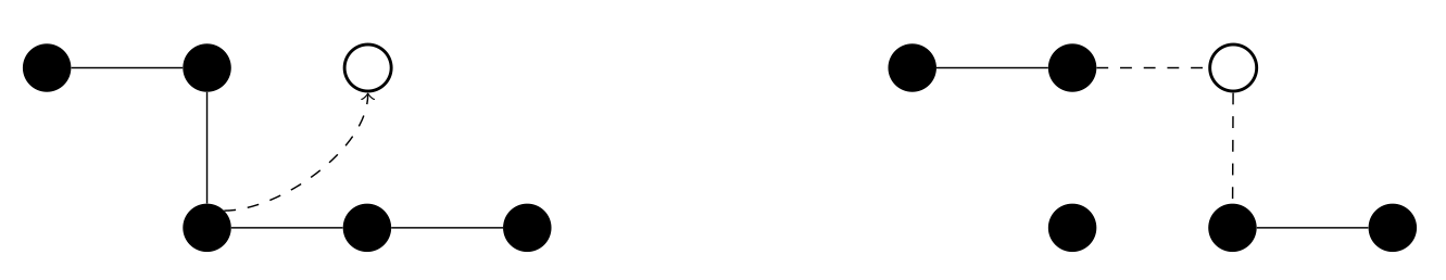
Figure 4: An example of a `bead flip' local move. The left image shows a fragment of the original conformation of a SAW, as determined by certain lattice points (filled circles). On changing one of these points to a new point (unfilled circle), a new conformation — not necessarily a SAW — is produced (right). Dashed lines show new features of the conformation resulting from the move.
Relatively speaking, local moves in MCMC methods have a low update cost and a high exploration cost. As a result, for large n they take an impractically long time to obtain a representative sample from the state space of cn n-step SAWs. Hence, if run time is limited, we will expect to obtain a sample for which many conformations have similar values of an observable.7 The problem is exacerbated as n becomes increasingly large. This feature limits the use of MCMC methods employing local moves to relatively small n as otherwise we are unlikely to obtain reasonable estimates of some observable.
We might expect that the increase in algorithm run time for very large n will be offset by ongoing increases in computing power. This rate of increase is well-established. In 1965 Moore observed that the number of transistors on an integrated circuit was increasing exponentially with time, doubling around every two years. Known as ‘Moore’s Law’, this rule of thumb remains a good approximation of how computing power increases over time. Since 1985, the number of transistors on a desktop computer has increased from approximately three hundred thousand to three billion. Computer hardware is also much cheaper than previously due to mass production. The overall result is an increase in computer power per dollar (neglecting the costs of electricity and maintenance) by a factor of the order of 10 million. This increase in computing power meant that researchers could use MCMC methods to obtain accurate estimates of observables of n-step SAWs for n of the order of hundreds. However, simulation for much larger n is required if we wish to gain insights into properties of polymers by estimating critical exponents. For these larger n, MCMC methods using local moves still have impractically long run times. Hence, hardware advances alone cannot enable the simulation of SAWs of a size that can push the frontiers of theoretical understanding.
The need to make algorithms faster stimulated further algorithm development.
Global moves in MCMC SAW simulation: a pivotal advance
The next generation of MCMC algorithms employed ‘global moves’ to deform SAW conformations. The pivot algorithm, invented by Lal in 1969 ([3]) and studied in depth by Madras and Sokal in 1988 ([4]), famously utilises a type of global move called a ‘pivot move’. A pivot move involves selecting a monomer at random (called the ‘pivot site’) and applying a transformation (most simply, a reflection or rotation) around that point. In terms of our pipe cleaner analogy, choosing a monomer about which to apply a move divides the SAW into two fragments, one on each side of the chosen monomer. One part of the SAW is held in place, this is the ‘stationary fragment’. The other, the ‘mobile fragment’, is bent or rotated around the chosen monomer (which itself does not move) without changing its shape so that it touches a different sequence of lattice points. Figure 5 shows an example of a pivot move that is a rotation.
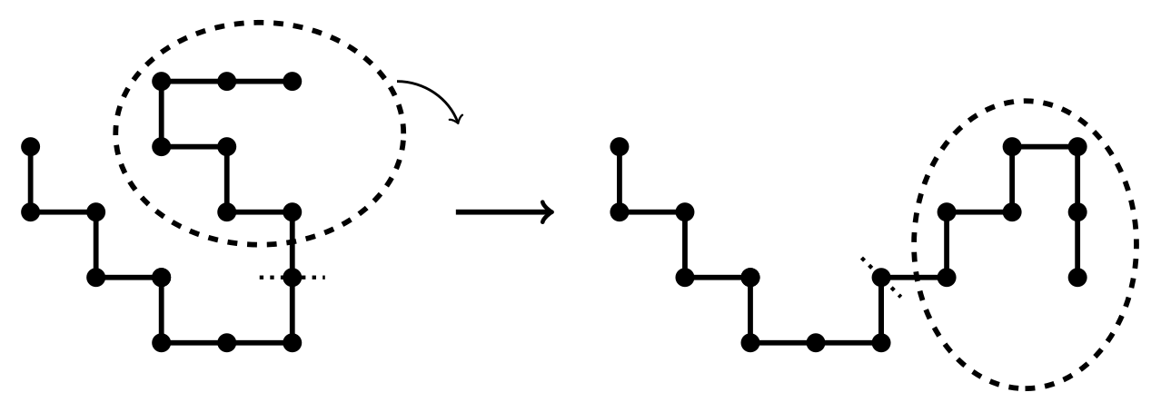
Figure 5: A SAW showing the mobile fragment enclosed by the dashed curve (left), and the SAW produced by application of a particular global move to the original conformation (right). The global move applied is a rotation of the mobile fragment 90 degrees to the right around the pivot site, the monomer indicated by the dotted line.
A global move applied to an n-step SAW tends to have a greater update cost than a local move applied for the same n for two reasons. First, a global move shifts a much greater number of monomers than a local move does.8 Second, deciding whether to accept or reject a global move requires checking more lattice points in the new conformation to determine whether it is a SAW. However, the distinct advantage of global moves over local moves is their lower exploration cost.9
The pivot algorithm improves algorithm run time by a factor that depends on n. Let us consider n = 109 (one billion) which is the number of monomers necessary for quantitative understanding of polymer knotting. In this case the speed up of SAW simulation algorithms is by a factor of 100 million. Speed up from the pivot algorithm made it possible to extend the simulation and useful calculation of properties of n-step SAWs from n of the order of hundreds to tens of thousands.
In 2002, Tom Kennedy [5] devised a means of significantly reducing the update cost of the pivot algorithm. This made it feasible to use simulation to accurately estimate observables of SAWs having hundreds of thousands or even millions of steps. However, the increase in algorithm run time with n still makes the standard algorithms unsuited to the very large n of practical interest.
Inspired by Kennedy’s contribution, Nathan considered how to further reduce the update cost in MCMC algorithms employing global moves. His original approach was to rethink the manner in which SAWs are represented on a computer. His efforts have greatly extended the usefulness of the pivot algorithm.
The breakthrough: think globally, act locally!
Nathan’s breakthrough followed an insight into the effect of a global move on a SAW configuration. A global move shifts each monomer in the mobile fragment to a new position in space. However, it does not change the fragment’s ‘shape’, that is, the relative positions of its monomers. Figure 5 illustrates this effect. The left figure shows a monomer directly above the pivot site in the original SAW conformation. The right figure shows that the global move shifts this monomer to the right of the pivot site. All other parts of the SAW’s shape are unchanged even though the global move causes a large change to the original configuration.
The conservation of features of a SAW’s shape by a global move has a useful consequence. In both the stationary and mobile fragments the SAW property is retained. Hence, it is only necessary to test whether the latter fragment intersects the former after the move. This reduces the amount of checking required by a MCMC algorithm in judging whether to accept or reject a move. Implementing this would result in an algorithm with a reduced update cost.
Nathan realised that storing fragment shapes — rather than monomer locations — was the key to this implementation. To achieve this he changed the data structure used from a table to a type of ‘binary tree’ he named the ‘SAW-tree’ (Clisby [6,7]).
A SAW-tree consists of cells arranged in levels. A cell contains the shape of a SAW fragment and aggregate information about its spatial extent. An example of a SAW-tree is shown in Figure 6. The top level has one cell containing the entire SAW conformation. This is divided into two fragments, with each assigned to a child cell at the next tree level. The similar application of this rule to each cell in a level causes the tree to grow downwards. The final level of the tree is reached when each cell contains the simplest type of fragment, one composed of two monomers.
The spatial information attached to each cell made it possible to decide rapidly that fragments do not overlap following the application of a global move to a conformation. This made it possible to check whether or not an entire conformation was a SAW more quickly than before. The SAW-tree also made it faster to update a stored SAW conformation as a result of a global move as this required relatively minor changes to the data structure. The combined effect was to reduce the update cost of a global move to that of a local move.
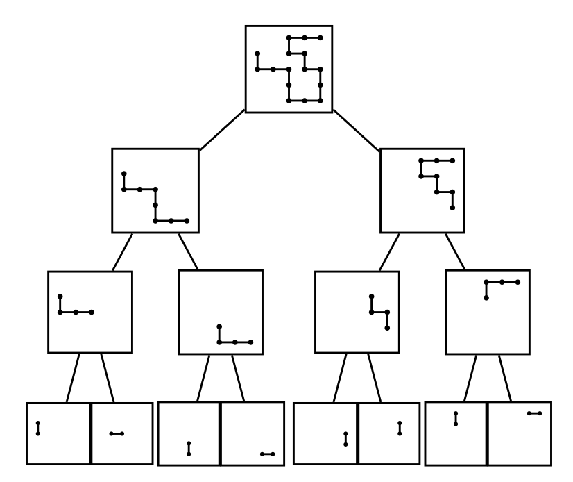
Figure 6: A SAW-tree representation of a self-avoiding walk.
Nathan’s MCMC algorithm for SAW simulation employing global moves and a SAW-tree data structure is clearly superior to earlier efforts. The use of global moves ensures a relatively low exploration cost whilst the new data structure results in a substantially lower update cost than the previous generation of MCMC algorithms. Testing Nathan’s algorithm against the test case of n-step SAWs with n = 109 steps showed a speed up of algorithm run time by a further factor of one million relative to the previous global-move MCMC algorithms on modern computers.
Comparison of Nathan’s algorithm against earlier algorithms for simulating SAW conformations illustrates the importance of this speed up. Nathan’s algorithm was used to sample 33 million step SAW conformations for about an hour of CPU time on a desktop computer. The estimates obtained for SAW observables (such as mean square length) had acceptably small error bars and were expected to be close to the true value in each case. It would take around seven years of CPU time to obtain comparably accurate estimates of observables using previous methods.
The future: SAW-trees and branching out into other complex computational problems
The improved efficiency achieved by Nathan’s algorithm has clear benefits for the study of SAWs. One concerns n-step SAWs for relatively small n. Researchers can revisit these to obtain more precise estimates of observables more quickly than before. Also, it is now possible to access a new regime in SAW simulation. One can routinely obtain good estimates of the properties of SAWs having hundreds of millions of monomers.10 This will enable a comparison of the prevalence of knots in large n-step SAWs with that detected in correspondingly large polymers (see Figure 7). The results will contribute to a greater understanding of how the features of polymer conformations change with the number of monomers. This may provide insight into questions such as how the presence of knotting influences DNA replication. The accurate estimates of observables obtained for various large n have already provided better quality inputs for the estimation of the critical exponents described earlier.
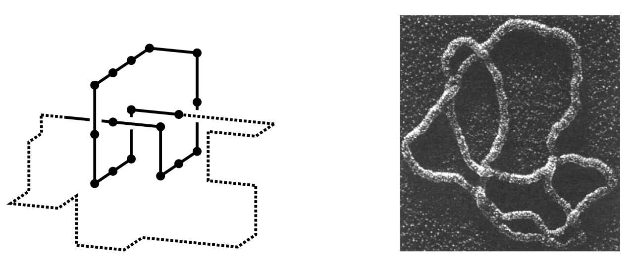
Figure 7: A knotted self-avoiding polygon (a SAW that forms a closed loop, left) and an electron micrograph of DNA showing a knot (right, image from Wasserman, Dungan, and Cozzarelli [8]).
Nathan’s SAW-tree algorithm also provides a general-purpose method for studying a wide range of other polymer problems. These include the study of the conformations of branched polymers and the behaviour of polymers confined between surfaces.
Many advances in mathematical research grow from an unique insight brought by an individual to their problem. Nathan’s original perspective on SAWs promises a fundamental contribution to the simulation of complex systems. Recall the key benefit of changing from the conventional data structure to the SAW-tree: a substantially lower update cost. This success suggests that customising a data structure to suit features of a particular system will similarly improve the efficiency of simulation algorithms employed. Nathan is currently working on applying the same underlying idea — i.e. fast data structures for global moves — to other models used in mathematical physics.
The development of powerful computer tools is akin to the invention of new instruments or techniques for physical experiments; both allow us to study new physical regimes. It is technically difficult to implement a software toolkit due to the complexity of the computer code required, and the corresponding ease of making mistakes in the programming effort. To ameliorate this, Nathan will be sharing his computer code in the near future. This will enable researchers to avoid ‘reinventing the wheel’ as they may adapt his software for their own problems.
- http://medical-treatment.org/95-frontallobe/244-frontallobe.html
-
T. K. Chaudhuri and S. Paul, Protein-misfolding diseases and chaperone-based therapeutic approaches, FEBS Journal 273:1331–1349, 2006.
-
M. Lal. ‘Monte Carlo’ computer simulation of chain molecules. Molecular Physics 17:57–64, 1969.
-
N. Madras and A. D. Sokal. The pivot algorithm: A highly efficient Monte Carlo method for the self-avoiding walk. Journal of Statistical Physics 50:109–186, 1988.
-
T. Kennedy. A faster implementation of the pivot algorithm for self-avoiding walks. Journal of Statistical Physics 106:407–429, 2002.
-
N. Clisby. Accurate estimate of the critical exponent ν for self-avoiding walks via a fast implementation of the pivot algorithm. Physical Review Letters 104:055702, 2010.
-
N. Clisby. Efficient implementation of the pivot algorithm for self-avoiding walks. Journal of Statistical Physics 140:349–392, 2010.
-
S. A. Wasserman, J. M. Dungan, and N. R. Cozzarelli. Discovery of a predicted DNA knot substantiates a model for site-specific recombination. Science 229:171–174, 1985.
Where ∼ is a shorthand for ‘behaves like’.↩
That is, the expression for cn may not be like — one that is written in terms of standard mathematical functions. Further, there might not even be an algorithm able to determine cn in polynomial time. Such an algorithm has a run time that is expected to be manageable even for very large n. It is greatly preferable to an exponential time algorithm for which run time increases drastically with n. This can make run time very long for relatively small n values, making the algorithm impractical for the much larger n values of interest.↩
For example, ‘lock and key’ models in which one protein’s conformation induces a change in that of another.↩
Briefly, a Markov chain is random process which is in one state of a state space at any instant of time. For any such state, there is some probability (possibly zero) of moving to any other state or remaining in the current state at any instant. A common application of Markov chains is in modelling a ‘birth and death’ process. The state space is the set of non-negative integers, representing the possible number of individuals in a population. At any instant there is some probability of certain events occurring. A birth (death) increases (decreases) the value of the state by one. If neither of these events occur, the state is unchanged. We will see the meaning of ‘Monte Carlo’ shortly.↩
The generation of a summary statistic (such as $\langle {\rm R^{2}_{e}} \rangle_n$) from samples drawn at random from a state space is a characteristic of ‘Monte Carlo’ methods.↩
Suppose we wish to estimate the average valuation of two bedroom houses in the metropolitan area of an Australian city. If we could determine the valuation of every house in this state space we would calculate the exact average valuation. As this is not practical, we must sample from the state space instead. Suppose we chose only to record the valuation of two bedroom houses in a prestigious suburb. These are likely to have valuations that are much more similar to each other than to houses picked at random from the metropolitan area. Also, their valuations are likely to be larger than those seen in many other suburbs in the city. As the sample of houses over-represents the more highly valued houses in the state space, it is not a representative sample. An average house valuation calculated from this unrepresentative sample is likely to substantially overestimate the actual average.↩
To continue the house valuation analogy used earlier, suppose we wished to explore the valuations of two bedroom houses by moving around a map at random. Suppose we start at a particular two bedroom house in our original expensive suburb. In this context, a local move is the equivalent of moving one house in any direction. The move is accepted if the new house has two bedrooms, and is rejected otherwise. It will take a relatively large number of moves to get out of our original suburb, and hence away from a region of similar house prices. We would expect the algorithm to take even more moves to get out of the relatively expensive inner-city suburbs and out to the considerably less expensive outer suburbs. Hence, an average house price computed for a relatively small number of moves will contain a disproportionate number of expensive homes, causing an overestimate of the average valuation.↩
Typically a substantial fraction of the total number of monomers is moved. This is most obvious when considering a global move applied around a monomer located away from the ends of a SAW.↩
Returning again to our house valuation problem, a global move is equivalent to moving from the current location to a randomly-selected house within a 10 km radius. An accepted move can potentially move us a large distance away from the previous two bedroom home.↩
Recall that this is the order of the number of monomers for which knots become prevalent in polymers.↩